Location estimate

Oelsnitz
Saxony · Germany
Approximate location reference—not a rooftop, property or survey point.
Seasonal average-day estimates
Selected capacity 1 kWp
Showing the original estimates at 1 kWp. JavaScript is needed only to change capacity; source values and panel settings remain available below.
Logarithmic slider: each labelled interval is 10× capacity. Energy scales linearly with capacity.
Arrow keys change capacity by about 2.3 percent per step. Page Up and Page Down move one labelled interval. Home selects 0.1 kWp; End selects 10 MWp.
Enter exact capacity and unit
Enter at least 0.1 kWp. Decimal point or comma; no thousands separators. 1 MWp = 1,000 kWp. Changing units keeps the same capacity. Exact entry keeps your precision; slider adjustments select three-significant-figure sizes.
There is no fixed upper capacity limit. Values and results must fit the calculator’s numeric range; the slider’s range is not an exact-entry limit.
Showing seasonal average-day estimates for 1 kWp.
Changing capacity rescales my existing estimates. It does not recalculate their orientation, shading, equipment or loss assumptions.
Estimated average daily electricity for 1 kWp, in kWh/day, averaged over each season.
Summer
kWh/day
Positive estimate rounded below 0.01 kWh/day display precision.
Autumn
kWh/day
Positive estimate rounded below 0.01 kWh/day display precision.
Winter
kWh/day
Positive estimate rounded below 0.01 kWh/day display precision.
Spring
kWh/day
Positive estimate rounded below 0.01 kWh/day display precision.
Very large results use scientific notation; an approximate capacity label is marked ≈. Exact capacity and full results remain available under Source basis and scaling limits.
Shared scale: 0–6.00 kWh/day.
I apply the same capacity factor to every season, so their proportions stay unchanged. The shared visual scale adjusts with capacity. To compare different system sizes, use the displayed kWh/day values.
This is illustrative scaling, not a site-specific production prediction.
Source basis and scaling limits
Original seasonal average-day estimates for Oelsnitz, in kWh/kWp/day.
I calculate the scaled results from the original seasonal values and round the final energy results to two decimal places. Exceptionally large values may appear in approximate scientific notation; the full results, rounded to two decimal places, remain available here.
| Season | Recorded kWh/kWp/day | Exact selected-capacity result · kWh/day |
|---|---|---|
| Summer | 5.16 | 5.16 × 1 kWp = 5.16 kWh/day |
| Autumn | 2.29 | 2.29 × 1 kWp = 2.29 kWh/day |
| Winter | 1.05 | 1.05 × 1 kWp = 1.05 kWh/day |
| Spring | 4.07 | 4.07 × 1 kWp = 4.07 kWh/day |
Ordinary calculations wrap onto two lines. Exceptionally long calculations can be scrolled within their labelled region.
Full results rounded to two decimal places
These preserve every whole-number digit. Exceptionally long values can be scrolled horizontally inside each labelled result.
- Summer · kWh/day
- 5.16
- Autumn · kWh/day
- 2.29
- Winter · kWh/day
- 1.05
- Spring · kWh/day
- 4.07
The original values remain available without JavaScript. Energy always uses kWh/day, including when capacity is entered in MWp. Changing units preserves the same physical capacity.
These are seasonal average-day estimates, not annual totals or installation sizing. Changing capacity does not revisit the assumptions used in my original estimates.
Detailed site analysisExplore historical generation and system configurations for your own project or your clients in the profileSOLAR app.
Year-round panel setup
- Tilt from horizontal
- 43°
- Facing direction
- South
Catalogue direction; exact azimuth not recorded. The facing direction is illustrative.
Suggested seasonal tilts
Tilt from horizontal · facing direction
- Summer
Jun, Jul, Aug - 34°South
- Autumn
Sep, Oct, Nov - 53°South
- Winter
Dec, Jan, Feb - 64°South
- Spring
Mar, Apr, May - 43°South
The seasonal electricity figures do not model gains from switching between these settings.
About this orientation
This schematic shows the year-round panel tilt and facing direction for Oelsnitz, Saxony, Germany.
For the year-round panel tilt, I used a simplified solar-noon calculation. This gives a broad starting point for considering a fixed panel angle at the location.
I weighted the daily angles by their share of estimated output. Read how I calculated panel tilt.
The panel shows tilt above horizontal on a fixed compass. North stays at the upper right in this projected view. Schematic only—not roof geometry, an installation drawing or a selected practical design.
Year-round and seasonal panel angles are separate estimates. Changing capacity rescales the existing energy values; it does not recalculate output for a different angle or facing direction.
Seasonal orientation diagrams
These show the separate seasonal settings above. Changing capacity does not change these angles or recalculate energy for a different orientation.
Summer
34° tilt · South
Illustrative direction; exact azimuth not recorded.
Autumn
53° tilt · South
Illustrative direction; exact azimuth not recorded.
Winter
64° tilt · South
Illustrative direction; exact azimuth not recorded.
Spring
43° tilt · South
Illustrative direction; exact azimuth not recorded.
 View larger
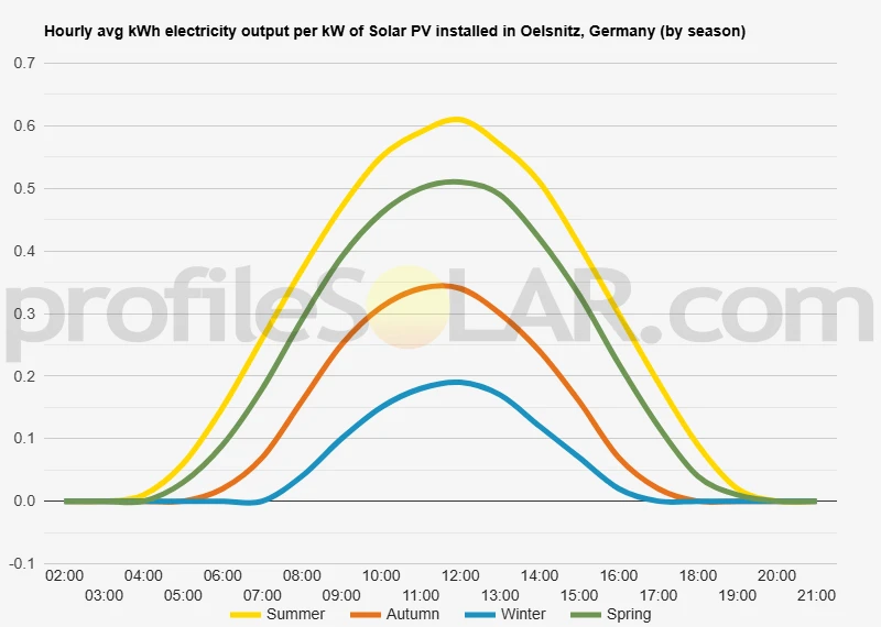
Hourly electricity pattern for Oelsnitz, Germany
Hourly profiles by season — Oelsnitz, Germany · 2021
This chart shows how average electricity output varies through the hours of the day in each season. I have kept its original per-capacity basis: changing the capacity slider does not change this chart.
2021 is the method’s reference year, not verified year coverage for every point in this historical chart.
The cards above show seasonal average-day energy; this chart shows the hourly pattern. View the year-round panel setup.
Row-spacing planning
Planning solar-panel row spacing in Oelsnitz
Explore the space between parallel panel rows at one assumed winter-solstice solar-noon position.
Example: 2 m panel surface length, recorded year-round tilt and no added margin. Enable JavaScript to change these inputs.
Panel and spacing inputs
Along the tilted surface, across the row. Greater than 0, up to 20 m; 2 m is an example.
Optional extra space, 0–100 m.
Starts at the recorded year-round tilt. Decimal entry is kept at your entered precision.
Linear slider: arrows select the next whole degree; Page Up/Down 10°, Home 0°, End 90°. Only moving it changes your numeric entry.
Results update automatically.
Example calculated with a 2 m panel surface length. Replace that example with the dimension of the module you are considering.
Example calculated with a 2 m panel surface length. Replace that example with the dimension of the module you are considering. Other published location estimates remain available.
Adjust the inputs to update this diagram and its results.
Row pitch including margin
≈ m
- Sunlight ray
- First row’s ground shadow
- Shadow endpoint
At this scale the panel surfaces are very small. The row labels locate them; exact dimensions remain available below.
- Calculated clear gap
- ≈ m
- Added margin
- ≈ 0 m
- Gap including margin
- ≈ m
- Panel horizontal footprint
- ≈ m
- Panel vertical rise
- ≈ m
- Pitch before margin
- ≈ m
Simplified level ground, equator-facing cross-section. Approximate Northern Hemisphere winter solstice at solar noon (day 355). The separate recorded facing direction is not an input.
One sun position, not a complete site-shading assessment. A geometric zero gap does not establish adequate installation, access or maintenance clearance.
Detailed inputs and unrounded results
More digits retain calculation precision; they do not imply greater model accuracy. Pitch including margin is pitch before margin plus the added margin, including when that margin is zero.
- Panel surface length
- 2 m
- Tilt up from horizontal
- 43°
- Added margin
- 0 m
- Latitude from the catalogue
- 50.717700000000000000° (Northern Hemisphere)
- Panel horizontal footprint
- 1.462707403238341 m
- Panel vertical rise
- 1.363996720124997 m
- Calculated clear gap
- 4.809841422428657 m
- Pitch before margin
- 6.272548825666998 m
- Gap including margin
- 4.809841422428657 m
- Row pitch including margin
- 6.272548825666998 m
- Design solar elevation
- 15.832517153186354°
How this spacing estimate is calculated
I calculate this example at approximate winter solstice and solar noon for the location’s hemisphere. Tilt is measured up from horizontal and panel length is measured along the tilted module surface.
δ = 23.45° × sin(360° × (day − 81) ÷ 365); α = asin(sin(latitude) × sin(δ) + cos(latitude) × cos(δ)).
Rise = length × sin(tilt). Footprint = length × cos(tilt). Clear gap = rise ÷ tan(α). Row pitch = footprint + clear gap. The optional margin is added to the gap and pitch.
The calculated clear gap is the horizontal distance from the first panel’s high edge to its shadow endpoint. Any added margin then extends to the next row. Pitch is measured between corresponding leading edges, not just across the clear gap. The target is no geometric shadow at that one simplified solar-noon design instant.
The cross-section assumes parallel, equator-facing rows and a solar-noon ray perpendicular to them. The method ignores azimuth error and does not use the separate facing direction recorded for this location.
Terrain, mounting height, module thickness, obstructions, structural loads and regulations are outside this simplified geometry. A qualified designer should verify a real installation.
Detailed site analysisExplore historical generation and system configurations for your own project or your clients in the profileSOLAR app.
Solar context for Oelsnitz
Read this location context alongside the calculation method and limitations; installation guidance is not a site-specific assessment.
Oelsnitz in the Erzgebirge has a marked summer-to-winter change in our solar estimate. Summer averages 5.16 kWh/day for each 1 kW of rated panel capacity, followed by spring at 4.07. Autumn is 2.29 and winter 1.05. For a household, the important implication is that useful spring and summer generation should be considered alongside a much smaller winter contribution.
Read the full article
Our year-round reference setting is 43° from horizontal facing South. We use it as a broad output-weighted angle for the location, not a guarantee of the best arrangement on a particular roof. The low winter figure is also a reason to examine consumption and supply across the year; it does not by itself determine the right battery size. Oelsnitz’s local energy landscape has a second dimension: coal mining has left a visible and underground legacy. The Deutschlandschachthalde is a spoil heap with a lookout tower and walking routes, while the former mining area is the subject of a state programme addressing mine-water recovery and other mining effects. This makes the town more distinctive than a general description of Ore Mountain foothills. An existing roof and a former mining surface should therefore be approached differently. For the roof, orientation, usable area and nearby obstructions are the starting questions. On previously worked ground, the history of the land and the current technical assessment matter alongside the available sunlight. A broad solar estimate cannot turn that history into a ready-made building site. Seasonal monitoring can help an owner judge whether an installed system follows its expected pattern. It is more useful to compare measured performance with conditions at the actual installation than to assume that a steeper angle, snow removal or a particular panel type will remove Oelsnitz’s winter shortfall.
Topography around Oelsnitz
These landscape descriptions provide general context. The calculations do not model terrain, obstructions, shading or property suitability.
Oelsnitz/Erzgebirge combines a small-valley setting with a strongly modified mining landscape. The Hegebach valley and former coal workings are important local features, as are the spoil heaps and reused industrial spaces. The municipal walking routes link the mining museum, the former garden-show grounds and the heap landscape, making that relationship visible on the ground.
Read the full topography description
The Deutschlandschachthalde is one of the town’s landmarks. It was created from coal-mining spoil and now has a lookout tower and recreational paths. The city’s account also describes continuing work on vegetation, slope stabilisation and rainwater routing there. Its shape and use should be understood as the outcome of mining and subsequent management, not as evidence of a flat vacant surface. Below ground, the Lugau–Oelsnitz coalfield has an extensive system of old workings. The Saxon mining authority explains that mine flooding has progressed since pumping ended and that effects on settlements, surface waters and landform require management. This is a specific reason to consult the relevant mining information before considering ground-based structures in the affected area. The wider landscape still includes residential streets, vegetation and changes in level. A site’s immediate horizon can differ from the view from a prominent heap or hill. Roof-based solar assessment can therefore focus on the building and its surroundings, while any land proposal should begin with its particular history and constraints. This description preserves Oelsnitz’s industrial and valley character. It does not rank northern fields or former mining land as preferred solar sites, and the local terrain has not been modelled as a shading adjustment in the catalogue estimate.
Technical location reference
Approximate map point used for Oelsnitz, Germany
This coordinate is the calculation reference for Oelsnitz, Germany. Extra decimal places do not make it a rooftop, property or survey point.
Coordinates and precision
- Map coordinate
- 50.717700000000000000, 12.728000000000000000
- Originally displayed coordinate
- lat50.7177 / long12.728
How the estimate works
How this Oelsnitz estimate was calculated
Here is how I calculated the location estimate for Oelsnitz, Germany.
Read how all Location estimates workSource and scope
I calculated these location estimates using hourly NASA POWER solar-resource data, with 2021 as the reference year. The seasonal figures show estimated daily electricity production averaged over each season, on a common panel-capacity basis.
The figures are calculated estimates, not measured output or a new NASA request while you browse.
Reference period and source details
The reference year describes the intended input period; complete source-year coverage is not established for every historical result. Read the technical questions about source data and downloads.
NASA POWER project reference
The data was obtained from National Aeronautics and Space Administration (NASA) Langley Research Center's Prediction Of Worldwide Energy Resources (POWER) project funded through the NASA Earth Science Division.
This source reference does not imply NASA endorsement.
Use the result carefully
What this Oelsnitz Location estimate includes and leaves out
Use the Oelsnitz figures for broad location context, with the following boundaries in mind.
- These catalogue estimates are informational; they do not establish a site-specific production result.
- The location is an approximate reference, not a property, rooftop or survey coordinate.
- The energy figures support broad location comparisons; they are not a generation guarantee or detailed system design.
- The seasonal cards show average-day energy. An hourly chart, where available, shows a different view of the daily pattern.
- Distance and clearance between rows require panel dimensions, mounting height, terrain, acceptable shading and a project-specific design.